Logistic Regression Algorithm Explained .
Logistic regression is a Binary Classification Algorithm , The Idea is very Simple we train The Model with a list of couples (x_i , y_i) to figure out The best Coefficient m and b that will fit our data .
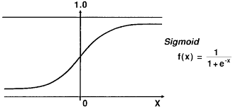
Then we apply an Activation Function called logistic Function or Sigmoid.
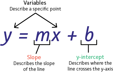
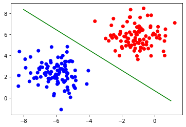
what we’re trying to do is we try to find A line ( Y = m*X + b ) that will split our data to two classes , class 0 where activation(Predicted value) >= 0.5 , class 1 where activation(Predicted value) < 0.5 .
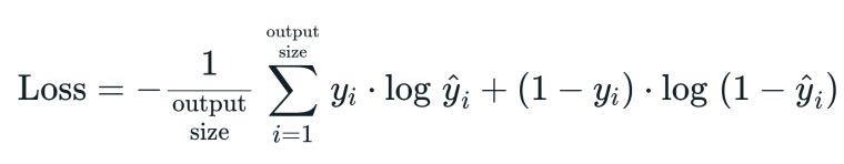
The Cost Function Used in this Example is Log-Loss and it defined as following :
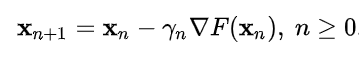
The Optimization Algorithm Used in this Example is Gradient Descent ans it defined as following :
Implementation :
1
2
3
4
5
6
7
8
9
10
11
12
13
14
15
16
17
18
19
20
21
22
23
24
25
26
27
28
29
30
31
32
33
34
35
36
37
38
39
40
41
42
43
44
45
46
47
48
49
50
51
52
53
54
55
56
57
58
59
60
61
62
63
64
import numpy as np
import matplotlib.pyplot as plt
from sklearn.datasets import make_blobs
from sklearn.model_selection import train_test_split
from sklearn.metrics import accuracy_score

class LogisticRegression :

    def __init__(self , learning_rate = 0.01 , nbr_iter = 1000):
        self.learning_rate = learning_rate
        self.nbr_iter = nbr_iter
        self.losses = []

    def initParameters(self , x):
        w = np.random.randn(x.shape[1])
        b = np.random.randn(1)
        return w , b
    def sigmoid(self,x):
        return 1 / (1 + np.exp(-x))

    def MSE(self , y_true , y_hat):
        return 1 / len(y_true) * np.sum((y_true - y_hat) ** 2)

    def fit(self , x , y):
        self.x_train = x
        self.y_train = y
        self.w , self.b = self.initParameters(self.x_train)

    def gradient(self,y_hat):
       dw = 1 / len(self.y_train) * -2 * np.dot(self.x_train.T , self.y_train - y_hat)
       db = 1 / len(self.y_train) * -2 * np.sum(self.y_train - y_hat)
       return dw , db

    def train(self):
        for i in range(self.nbr_iter) :
            z = np.dot(self.x_train , self.w) + self.b
            y_hat = self.sigmoid(z)
            loss = self.MSE(self.y_train , y_hat)
            self.losses.append(loss)
            dw , db = self.gradient(y_hat)

            self.w -= self.learning_rate * dw
            self.b -= self.learning_rate * db

    def predict(self , x):
        z = np.dot(x , self.w) + self.b
        y_hat = self.sigmoid(z)
        y_hat = [1 if yi >= 0.5 else 0 for yi in y_hat]
        return np.array(y_hat)

    def didplayTheModel(self , x , y):
        x1 = np.linspace(0 , 100 , self.nbr_iter)
        plt.plot(x1 , self.losses)
        plt.title("Loss")
        plt.show()

        fig , ax = plt.subplots()
        x0_lim = ax.get_xlim()

        ax.scatter(x[:,0] , x[:,1] , c = y , cmap="bwr")
        x1 = np.linspace(-8,x0_lim[1],200)
        x2 = (-x1 * self.w[0]   - self.b) / self.w[1]
        plt.plot(x1  , x2 , c='g')
        plt.show()
Test The Model :
1
2
3
4
5
6
7
8
9
x , y = make_blobs(n_samples=200 , n_features=2 , centers= 2 , random_state=1234)
x_train , x_test , y_train , y_test = train_test_split(x , y , test_size=0.25)

L_regression = LogisticRegression()
L_regression.fit(x_train, y_train)
L_regression.train()
y_hat = L_regression.predict(x_test)
score = accuracy_score(y_test , y_hat)
L_regression.didplayTheModel(x, y)
The Model Result :
The Loss of The Model :
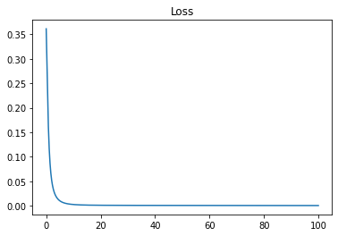
In this example we used 100 iteration to train The Model , and as you can see The Loss is decreasing Over iterations .